As mentioned in the statistics day with with Amy Willis and Maria Valdez-Cabrera the genomics experiment can be divided in two main sections:
- The data reduction from raw FASTQ files to some count tables (bioinformatics)
- The statistical analysis of those count tables (inferential statistics)
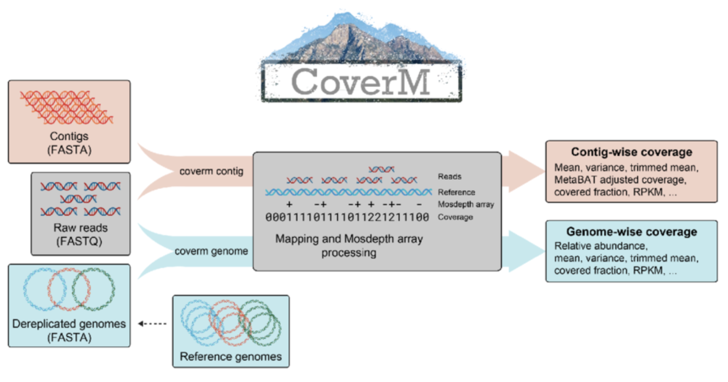
The mapping of reads against the co-assembly allows us to quantify the coverage of each contig in each sample (something you are very familiar with, thanks to Anvi’o).
We can use CoverM to produce an abundance table from a set of BAM files.
Installing CoverM
We installed CoverM inside the “mapping” conda environment, otherwise it’s easy installable from BioConda.
# Activate the environment
conda activate mapping

# Check installation
coverm --version
Running CoverM
We have three BAM files in bams/, each corresponding to the mapping of one sample against the co-assembly.
# Calculate coverage metrics for all contigs
coverm contig \
  -b /*.bam \
  -m count mean covered_fraction tpm \
  -o abundance_table.tsv \
  --exclude-supplementary \
  -t 8
Some explanations about the parameters used:
-
contig: is a subcommand which tells CoverM to calculate metrics at the contig level -
-b: specifies the input BAM files (you can specify multiple files, also using wildcards) -
-m: specifies the metrics to calculate, in this case:-
count: the number of reads mapped to the contig -
mean: mean coverage depth across the contig -
covered_fraction: proportion of contig covered by reads (0-1) -
tpm: Transcripts Per Million (normalized abundance)
-
-
-o: specifies the output file name -
--exclude-supplementary: excludes supplementary alignments from the calculations -
-t: number of threads to use
Output File
The output is a TSV file with the following structure:
| Column | Description |
|---|---|
| Contig | Contig identifier |
| {Sample} Count | Number of reads mapped to the contig |
| {Sample} Mean | Mean coverage depth across the contig |
| {Sample} Covered Fraction | Proportion of contig covered by reads (0-1) |
| {Sample} TPM | Transcripts Per Million (normalized abundance) |
Each sample gets one column per requested metric. In this case, with 3 samples and 4 metrics, you’ll have 13 columns total (1 for contig names + 3 samples × 4 metrics).
Note: Raw counts are the most useful value to perform statistical analyses, while TPM values are useful for a first “eyeballing” comparison of abundances between samples, as they account for both sequencing depth and contig length.