Introduction to qipalette • qipalette

library(qipalette)

Overview

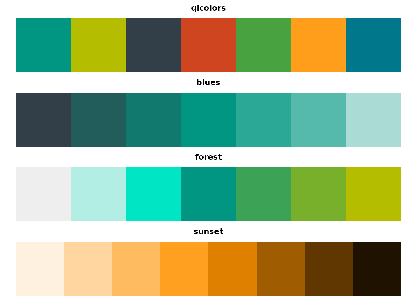
The qipalette package provides a collection of color palettes for data visualization in R, inspired by the branding colors of the Quadram Institute Bioscience. This vignette demonstrates how to use the package functions and apply the palettes to your visualizations.

Available Palettes

Let’s start by displaying all available palettes:

display_all_palettes()

Basic Usage

Getting Colors from a Palette

You can extract colors from a palette using the get_palette() function:

# Get the default number of colors
sunset_colors <- get_palette("qicolors")
sunset_colors
#> [1] "#009681" "#B5BD00" "#333F48" "#CF4520" "#48A23F" "#FF9E1B" "#00778B"

# Get a specific number of colors
sunset_colors_8 <- get_palette("sunset", n = 8)
sunset_colors_8
#> [1] "#fff1df" "#ffd69f" "#ffbb60" "#ffa020" "#df8000" "#9f5c00" "#603700"
#> [8] "#201200"

# Reverse the palette
sunset_colors_rev <- get_palette("sunset", reverse = TRUE)
sunset_colors_rev
#> [1] "#201200" "#603700" "#9f5c00" "#df8000" "#ffa020" "#ffbb60" "#ffd69f"
#> [8] "#fff1df"

Using with Base R Graphics

The palettes can be easily used with base R graphics:

# Scatter plot with colors by group
plot(1:5, 1:5, col = get_palette("qicolors", 5), pch = 19, cex = 3,
     main = "qicolors Palette Demo", xlab = "X", ylab = "Y")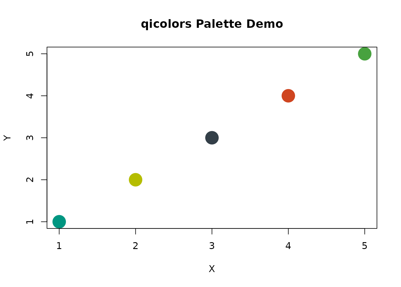


# Bar plot
barplot(1:5, col = get_palette("blues"), main = "blues Palette Demo")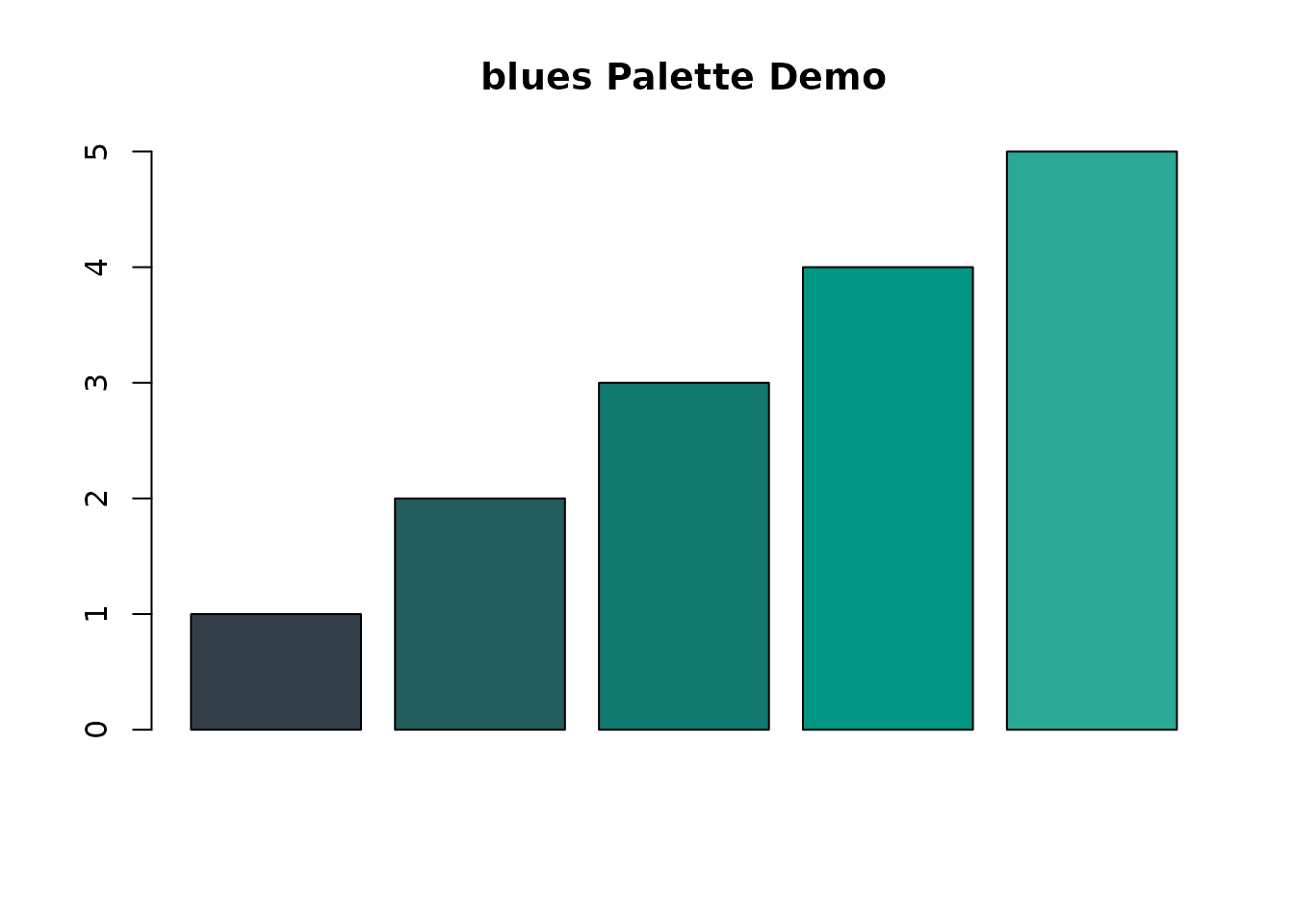


# Pie chart
pie(rep(1, 5), col = get_palette("forest"), main = "forest Palette Demo")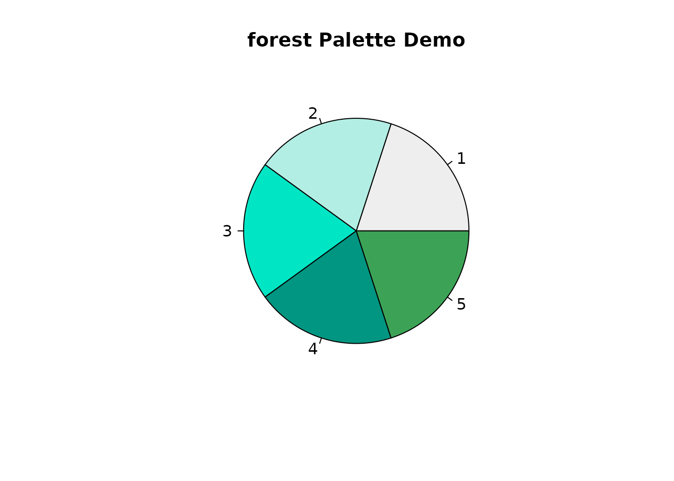

Integration with ggplot2

The package includes functions for easy integration with ggplot2:

library(ggplot2)

# Scatter plot with discrete color scale
ggplot(mtcars, aes(wt, mpg, color = factor(cyl))) +
  geom_point(size = 3) +
  scale_color_palette("blues") +
  labs(title = "Car Weight vs MPG", color = "Cylinders")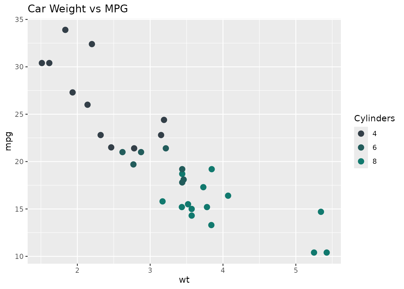


# Bar plot with fill scale
ggplot(data.frame(x = letters[1:5], y = 1:5), aes(x, y, fill = x)) +
  geom_col() +
  scale_fill_palette("qicolors") +
  labs(title = "Sample Bar Chart", fill = "Category")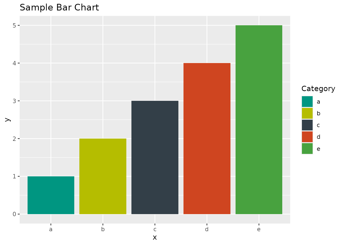

Advanced Usage

Continuous Color Scales

For continuous variables, you can set discrete = FALSE:

ggplot(faithfuld, aes(waiting, eruptions, fill = density)) +
  geom_tile() +
  scale_fill_palette("sunset", discrete = FALSE) +
  labs(title = "Old Faithful Eruption Density")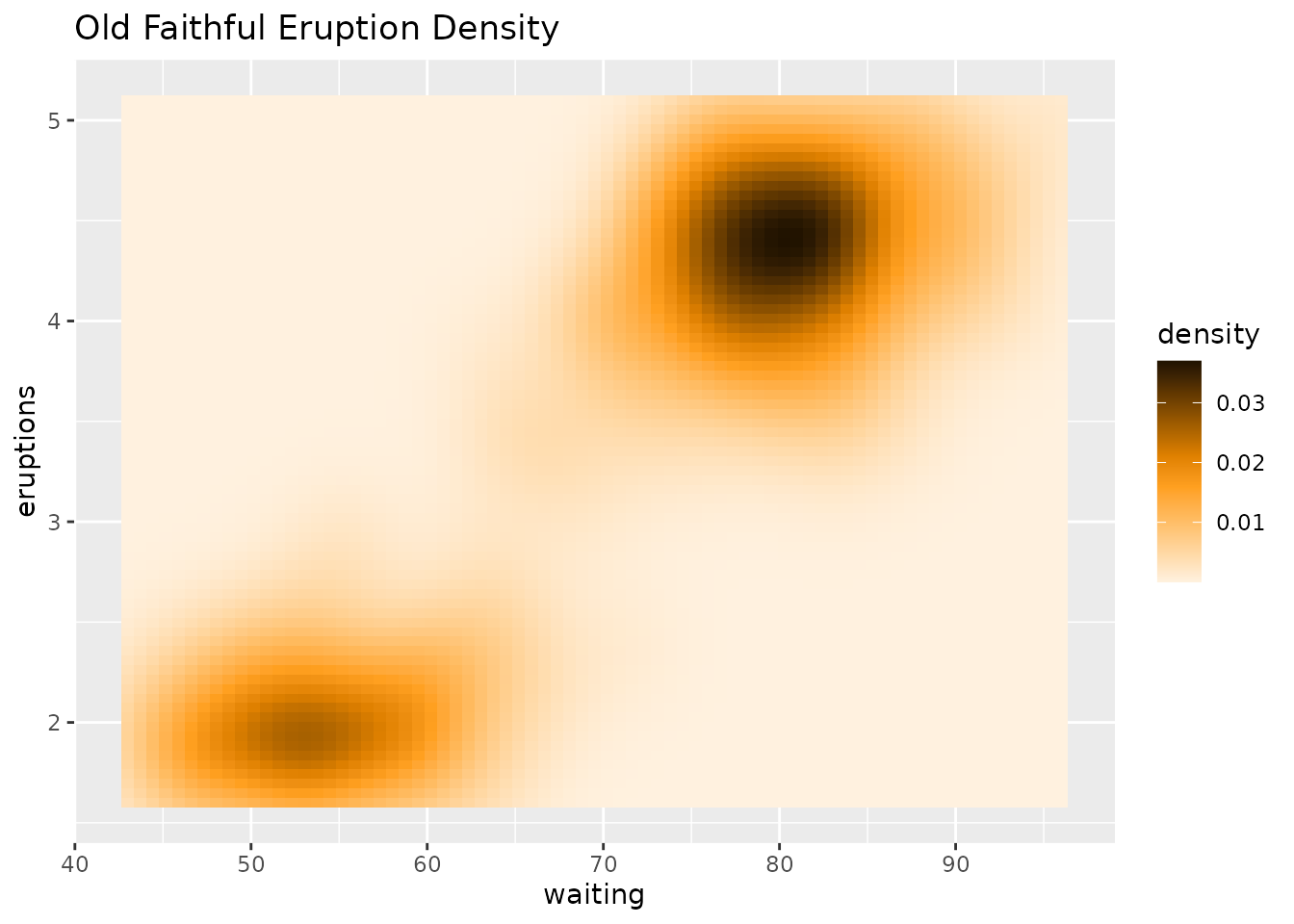

Custom Plotting Function

You can use the palette_color() function for flexible coloring based on categories:

# Create a factor variable
groups <- factor(rep(letters[1:3], each = 5))

# Plot with palette_color
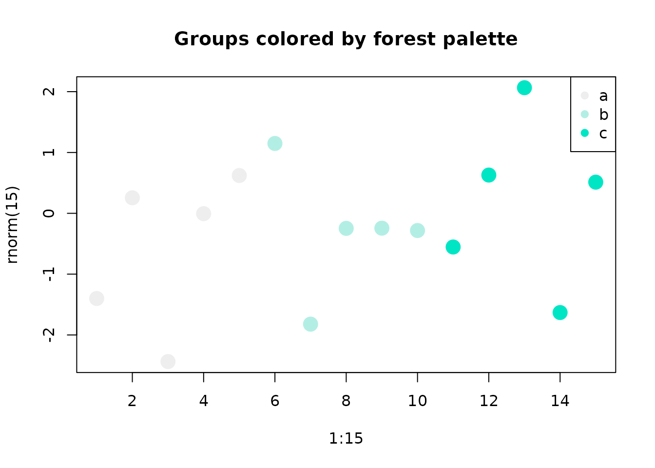
plot(1:15, rnorm(15), col = palette_color("forest")(groups), pch = 19, cex = 2,
     main = "Groups colored by forest palette")
legend("topright", legend = levels(groups),
       col = get_palette("forest", 3), pch = 19)