Keep in mind the statistics day with Amy Willis and Maria Valdez-Cabrera: a genomics experiment can be divided in two main sections:

• The data reduction from raw FASTQ files to some count tables (bioinformatics)
• The statistical analysis of those count tables (inferential statistics)

The mapping of reads against the co-assembly allows us to quantify the coverage of each contig in each sample (something you are very familiar with, thanks to Anvi’o).

What is coverage, again?

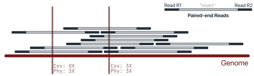
Coverage (or depth) is the number of reads overlapping a given position of the reference. It is a per-base measure: each position of a contig has its own coverage value, and these values can be summarised (e.g. mean or median coverage of a contig).

Physical coverage counts the whole sequenced fragment rather than the individual reads. With paired-end data, the unsequenced gap between the two mates is also considered covered, because we know a DNA molecule spanned that region. Physical coverage is therefore always equal to or higher than sequence coverage, and is useful to check whether a region is supported by intact fragments (e.g. when assessing assembly joins).

Counts are something different: the number of reads assigned to a feature (a contig, a gene, a genome), with no information on where they map. Counts depend on the length of the target: a long contig collects more reads than a short one at the same abundance. Coverage is implicitly normalised by length, which makes it a better proxy for abundance when comparing targets of different sizes.

Two contigs with the same number of reads can have very different coverage profiles, and the same mean coverage can hide very different situations. This is why we also look at:

• Breadth of coverage: the fraction of the reference covered by at least one read (or above a chosen threshold).
• Coverage uniformity: how evenly reads are distributed along the reference. A genome that is genuinely present should be covered fairly evenly; reads piling up on a short region (e.g. a conserved gene shared by related viruses) while the rest is uncovered usually indicate a spurious or partial hit rather than true presence.

It starts with mapping

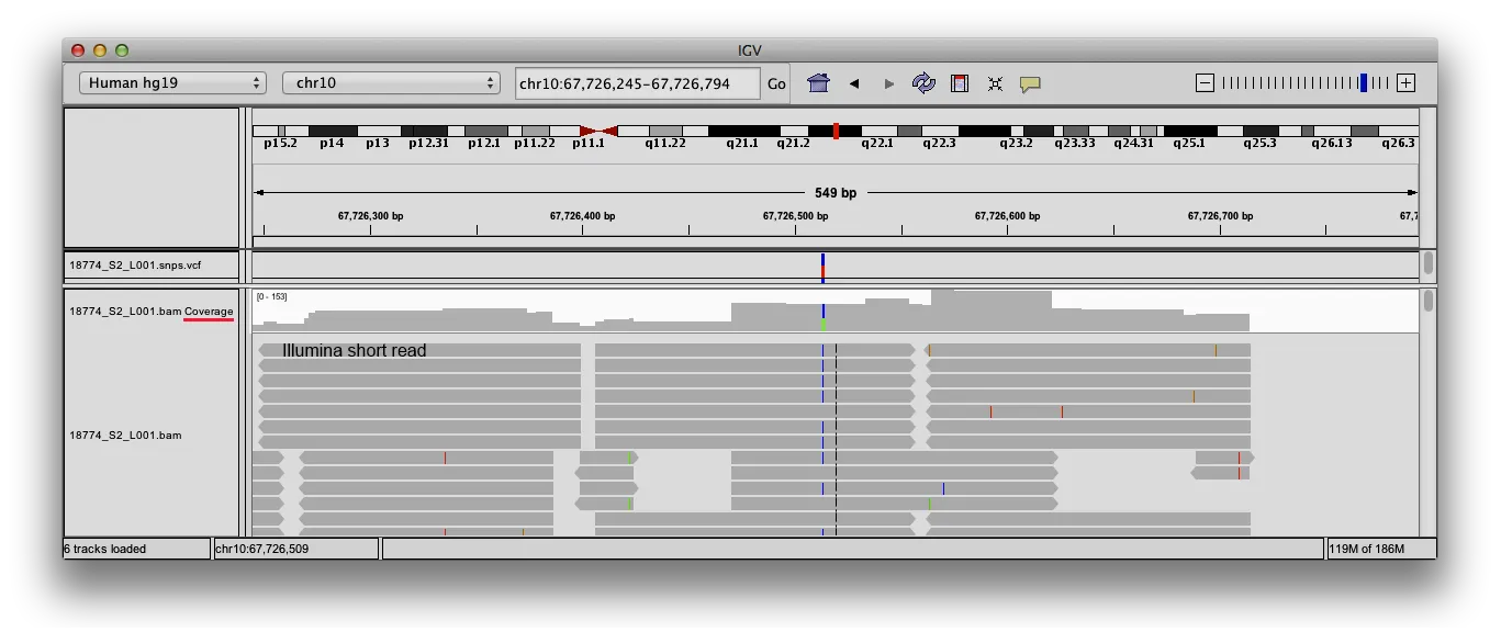
Coverage can be visualised with IGV (see screenshot above).

Coverage is calculated from an alignment file in BAM format, produced by mapping the reads against a reference (e.g. a set of viral contigs). The BAM file should be sorted by coordinate (and indexed).

Not all the alignments in a BAM file are equal, and some choices affect which ones contribute to coverage:

• Mapping quality (MAPQ): reads that map equally well to multiple places receive a low MAPQ. In viromes, where related genomes share similar regions, filtering by MAPQ can noticeably change the coverage of some contigs.
• SAM flags: unmapped, secondary, supplementary, duplicate or QC-failed alignments are normally excluded, but the tool settings determine this.
• Alignment details: soft-clipped bases and deletions may or may not be counted as covered, depending on the tool.

When comparing coverage values, always make sure they were computed with the same filters.

---