Denoising with DADA2
The core DADA2 algorithm uses the error model learned in the previous chapter to distinguish true biological sequences from sequences that arose through PCR or sequencing errors. It works by asking: given the error model, is this slightly different sequence more likely to be a genuine variant, or an error-derived copy of a more abundant sequence?
The result is a set of Amplicon Sequence Variants (ASVs) : exact sequences with no artificial clustering.
dadaFs_file <- file.path ( path_precomp , "dadaFs.rds" ) dadaRs_file <- file.path ( path_precomp , "dadaRs.rds" ) if ( ! file.exists ( dadaFs_file ) ) { message ( "Denoising forward reads..." )
dadaFs <- dada ( filtFs , err = errF , multithread = TRUE )
saveRDS ( dadaFs , dadaFs_file )
} else { dadaFs <- readRDS ( dadaFs_file )
}
Sample 1 - 13226 reads in 4843 unique sequences.
Sample 2 - 178641 reads in 22804 unique sequences.
Sample 3 - 12109 reads in 4696 unique sequences.
Sample 4 - 1419 reads in 581 unique sequences.
Sample 5 - 34239 reads in 11798 unique sequences.
Sample 6 - 193289 reads in 26735 unique sequences.
Sample 7 - 221122 reads in 21753 unique sequences.
Sample 8 - 150467 reads in 15443 unique sequences.
Sample 9 - 189922 reads in 24078 unique sequences.
Sample 10 - 227640 reads in 22363 unique sequences.
Sample 11 - 210626 reads in 20738 unique sequences.
Sample 12 - 191040 reads in 24153 unique sequences.
Sample 13 - 233210 reads in 29369 unique sequences.
Sample 14 - 107509 reads in 25626 unique sequences.
Sample 15 - 219755 reads in 23609 unique sequences.
Sample 16 - 213873 reads in 22116 unique sequences.
Sample 17 - 230240 reads in 29372 unique sequences.
Sample 18 - 209712 reads in 42650 unique sequences.
Sample 19 - 241630 reads in 45010 unique sequences.
Sample 20 - 209072 reads in 36916 unique sequences.
Sample 21 - 253245 reads in 32445 unique sequences.
Sample 22 - 243119 reads in 43825 unique sequences.
Sample 23 - 238579 reads in 37930 unique sequences.
Sample 24 - 217397 reads in 41176 unique sequences.
Sample 25 - 218668 reads in 39233 unique sequences.
Sample 26 - 239236 reads in 43927 unique sequences.
Sample 27 - 237723 reads in 42642 unique sequences.
Sample 28 - 208982 reads in 43512 unique sequences.
Sample 29 - 256480 reads in 44096 unique sequences.
if ( ! file.exists ( dadaRs_file ) ) { message ( "Denoising reverse reads..." )
dadaRs <- dada ( filtRs , err = errR , multithread = TRUE )
saveRDS ( dadaRs , dadaRs_file )
} else { dadaRs <- readRDS ( dadaRs_file )
}
Sample 1 - 13226 reads in 6970 unique sequences.
Sample 2 - 178641 reads in 28216 unique sequences.
Sample 3 - 12109 reads in 6149 unique sequences.
Sample 4 - 1419 reads in 729 unique sequences.
Sample 5 - 34239 reads in 15345 unique sequences.
Sample 6 - 193289 reads in 32391 unique sequences.
Sample 7 - 221122 reads in 29710 unique sequences.
Sample 8 - 150467 reads in 22351 unique sequences.
Sample 9 - 189922 reads in 30935 unique sequences.
Sample 10 - 227640 reads in 29549 unique sequences.
Sample 11 - 210626 reads in 28342 unique sequences.
Sample 12 - 191040 reads in 33939 unique sequences.
Sample 13 - 233210 reads in 35191 unique sequences.
Sample 14 - 107509 reads in 18547 unique sequences.
Sample 15 - 219755 reads in 31439 unique sequences.
Sample 16 - 213873 reads in 29943 unique sequences.
Sample 17 - 230240 reads in 36340 unique sequences.
Sample 18 - 209712 reads in 53263 unique sequences.
Sample 19 - 241630 reads in 55632 unique sequences.
Sample 20 - 209072 reads in 47285 unique sequences.
Sample 21 - 253245 reads in 41514 unique sequences.
Sample 22 - 243119 reads in 59760 unique sequences.
Sample 23 - 238579 reads in 52820 unique sequences.
Sample 24 - 217397 reads in 51954 unique sequences.
Sample 25 - 218668 reads in 49783 unique sequences.
Sample 26 - 239236 reads in 54978 unique sequences.
Sample 27 - 237723 reads in 49322 unique sequences.
Sample 28 - 208982 reads in 52167 unique sequences.
Sample 29 - 256480 reads in 55448 unique sequences.
What does the dada2 output tell us?
# Inspect the first sample's denoising result dadaFs [[ 1 ] ]
dada-class: object describing DADA2 denoising results
90 sequence variants were inferred from 4843 input unique sequences.
Key parameters: OMEGA_A = 1e-40, OMEGA_C = 1e-40, BAND_SIZE = 16
The output reports how many unique sequences were identified in the sample and how many reads support each one. The ratio of reads to unique sequences gives an indication of how much error correction was performed.
Merging paired-end reads
After denoising, forward and reverse reads are merged to reconstruct the full amplicon sequence. Merging requires a minimum overlap region between the denoised forward and reverse reads — by default, at least 12 bp.
mergers_file <- file.path ( path_precomp , "mergers.rds" ) if ( ! file.exists ( mergers_file ) ) { message ( "Merging paired reads..." )
mergers <- mergePairs ( dadaFs , filtFs , dadaRs , filtRs , verbose = TRUE )
saveRDS ( mergers , mergers_file )
} else { mergers <- readRDS ( mergers_file )
}
If a large proportion of reads fail to merge (visible in the tracking table later), the most common causes are:
Insufficient overlap — increase truncLen for one or both reads, or reduce it if the reads are too short
Primer residues — verify that primers were fully removed before this analysis
Wrong amplicon size — the reads must cover the amplicon with some overlap
Build the sequence table
makeSequenceTable() produces a sample × ASV matrix of read counts. This is the central data object in DADA2.
seqtab <- makeSequenceTable ( mergers ) cat ( "Dimensions (samples × ASVs):" , dim ( seqtab ) , "\n" )
Dimensions (samples × ASVs): 29 18934
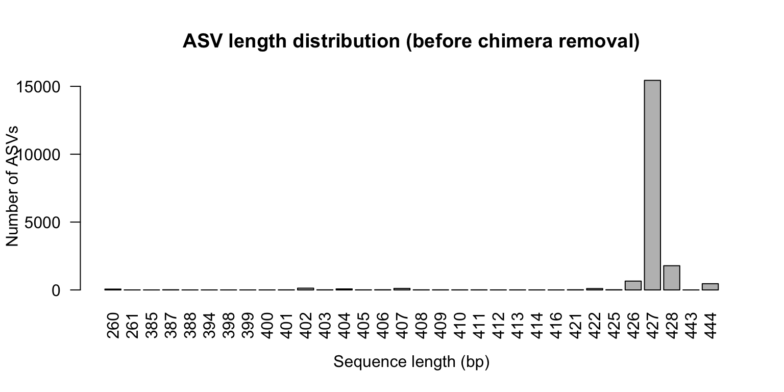
Sequence length distribution
The expected amplicon length for the V3–V4 region is approximately 400–470 bp. Any sequences outside this range are likely artefacts (non-specific amplification or chimeras) and will often be removed in subsequent steps.
  260   261   385   387   388   394   398   399   400   401   402   403   404
   62     2     1    12     1     1     1     1     2     5   132     8    75
  405   406   407   408   409   410   411   412   413   414   416   421   422
    5    12   112     7     7     5     6     3     4     3     2    12   102
  425   426   427   428   443   444
   13   652 15440  1785     2   459
# Visualise barplot ( seq_lengths , xlab = "Sequence length (bp)" ,
ylab = "Number of ASVs" ,
main = "ASV length distribution (before chimera removal)" ,
las = 2 )
Chimera removal
Chimeric sequences are PCR artefacts created when an incomplete extension product from one cycle acts as a primer in a subsequent cycle, fusing the 5′ end of one template with the 3′ end of another. DADA2 identifies chimeras using the removeBimeraDenovo() function, which checks whether each sequence can be reconstructed from two more-abundant “parent” sequences.
seqtab_file <- file.path ( path_precomp , "seqtab_nochim.rds" ) if ( ! file.exists ( seqtab_file ) ) { message ( "Removing chimeras..." )
seqtab.nochim <- removeBimeraDenovo ( seqtab ,
method = "consensus" ,
multithread = TRUE ,
verbose = TRUE )
saveRDS ( seqtab.nochim , seqtab_file )
} else { seqtab.nochim <- readRDS ( seqtab_file )
} cat ( "ASVs before chimera removal:" , ncol ( seqtab ) , "\n" )
ASVs before chimera removal: 18934
cat ( "ASVs after chimera removal:" , ncol ( seqtab.nochim ) , "\n" )
ASVs after chimera removal: 1091
pct_retained <- round ( 100 * sum ( seqtab.nochim ) / sum ( seqtab ) , 1 ) cat ( "Proportion of reads retained after chimera removal:" , pct_retained , "%\n" )
Proportion of reads retained after chimera removal: 89.8 %
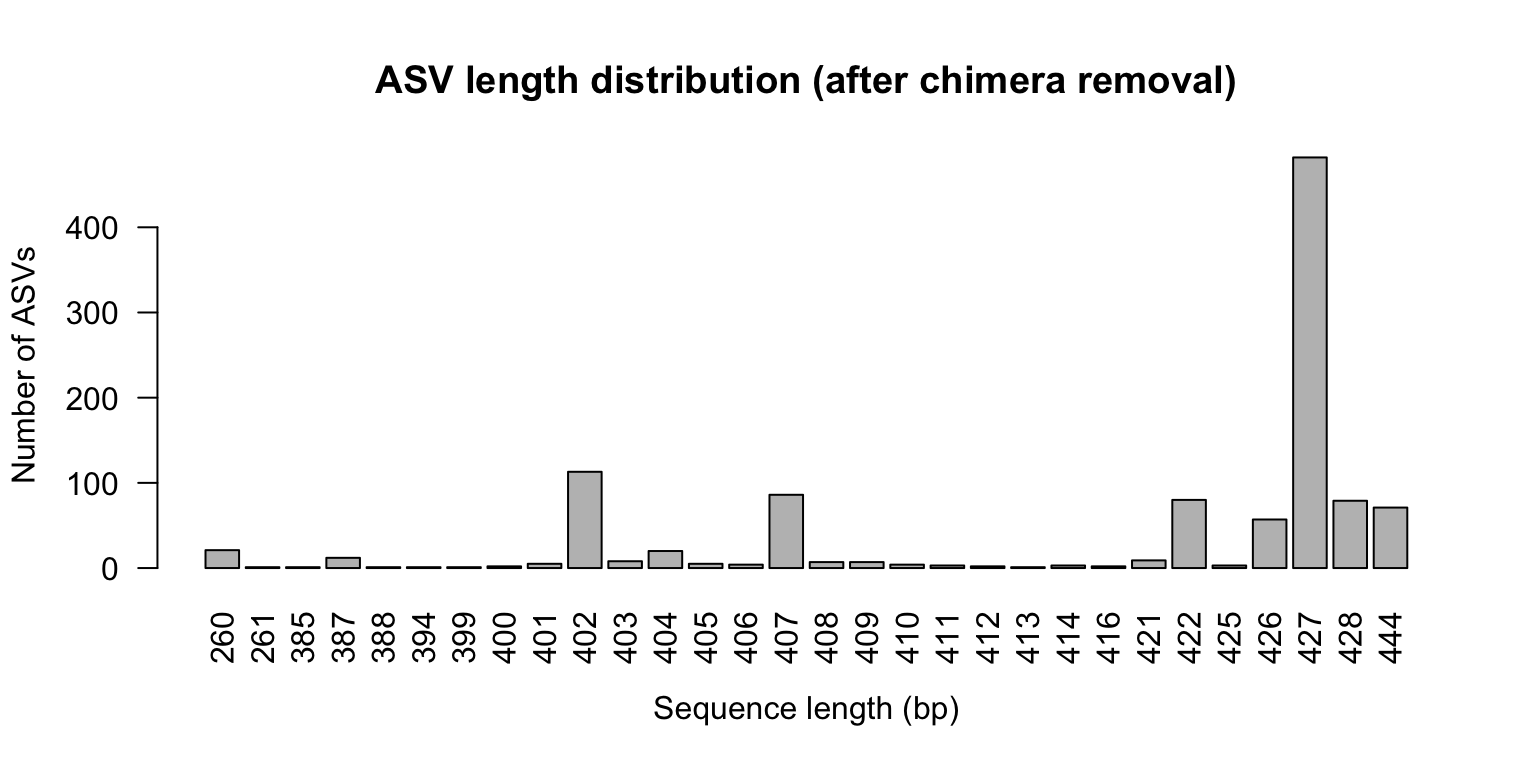
It is normal for a large number of unique sequences to be flagged as chimeric — often 10–30 % of ASVs. However, chimeric reads usually represent a small proportion of total reads (< 10 %), because chimeras are typically rare relative to their parent sequences. If you lose > 20 % of reads here, double-check that primers were fully trimmed.
seq_lengths_nc <- table ( nchar ( getSequences ( seqtab.nochim ) ) ) print ( seq_lengths_nc )
260 261 385 387 388 394 399 400 401 402 403 404 405 406 407 408 409 410 411 412
 21   1   1  12   1   1   1   2   5 113   8  20   5   4  86   7   7   4   3   2
413 414 416 421 422 425 426 427 428 444
  1   3   2   9  80   3  57 482  79  71
barplot ( seq_lengths_nc , xlab = "Sequence length (bp)" ,
ylab = "Number of ASVs" ,
main = "ASV length distribution (after chimera removal)" ,
las = 2 )
Tracking reads through the pipeline
A key quality-control step is to track how many reads survive each stage of the pipeline. Large losses at any single step point to a specific problem.
getN <- function ( x ) sum ( getUniques ( x ) ) track <- cbind ( out ,
denoisedF = sapply ( dadaFs , getN ) ,
denoisedR = sapply ( dadaRs , getN ) ,
merged = sapply ( mergers , getN ) ,
nonchim = rowSums ( seqtab.nochim )
) colnames ( track ) <- c ( "input" , "filtered" , "denoisedF" , "denoisedR" , "merged" , "nonchim" )
rownames ( track ) <- sample.names write.csv ( track , "dada2_QC.csv" ) track
                      input filtered denoisedF denoisedR merged nonchim
Commercial_R1         16778    13226     13183     13200  13113   12499
Commercial_R2        218777   178641    177733    178459 176766  176479
Commercial_R3         14993    12109     12049     12098  11922   11670
Control_extraction     2345     1419      1411      1414   1403    1403
Control_fermentation  42709    34239     34114     34105  33515   33162
Lactobacillus_H24_R1 236996   193289    192552    192803 190009  178597
Lactobacillus_H24_R2 271744   221122    220906    220980 220054  217351
Lactobacillus_H24_R3 185402   150467    150220    150328 149791  148672
Lactobacillus_H48_R1 232087   189922    189536    189665 187248  177255
Lactobacillus_H48_R2 277388   227640    227197    227476 226648  222104
Lactobacillus_H48_R3 257945   210626    210217    210457 209083  205846
Lactobacillus_W1_R1  237242   191040    190633    190702 189362  185573
Lactobacillus_W1_R2  283367   233210    232746    232883 230755  224196
Lactobacillus_W1_R3  135637   107509    107352    107386 106982  105252
Lactobacillus_W2_R1  270194   219755    219374    219573 218558  217417
Lactobacillus_W2_R2  262219   213873    213132    213708 212577  209841
Lactobacillus_W2_R3  280448   230240    229271    229942 227359  218116
Spontaneous_H24_R1   260410   209712    208384    208726 197139  162260
Spontaneous_H24_R2   297828   241630    240341    240755 230290  169513
Spontaneous_H24_R3   258467   209072    208224    208561 202745  166417
Spontaneous_H48_R1   311391   253245    252497    252931 229750  203601
Spontaneous_H48_R2   302367   243119    241992    242408 232963  186846
Spontaneous_H48_R3   295072   238579    237584    238146 230008  193478
Spontaneous_W1_R1    266958   217397    216521    216709 206641  165163
Spontaneous_W1_R2    271112   218668    218010    217981 207723  180948
Spontaneous_W1_R3    295075   239236    238162    238617 230440  187702
Spontaneous_W2_R1    291669   237723    236868    237129 225123  190377
Spontaneous_W2_R2    259494   208982    208097    208521 200762  151955
Spontaneous_W2_R3    314666   256480    255722    255872 248160  210209
Visualise read tracking
step_labels <- c ( input = "Raw Input" ,
filtered = "Quality Filtered" ,
denoisedF = "Denoised (Fwd)" ,
denoisedR = "Denoised (Rev)" ,
merged = "Merged Pairs" ,
nonchim = "Non-chimeric"
) track_long <- as.data.frame ( track ) %>% rownames_to_column ( "Sample" ) %>%
pivot_longer ( - Sample , names_to = "Step" , values_to = "Reads" ) %>%
mutate ( Step = factor ( Step , levels = names ( step_labels ) ) )
ggplot ( track_long , aes ( x = Step , y = Reads , fill = Step ) ) + geom_boxplot ( outlier.size = 1 ) +
scale_x_discrete ( labels = step_labels ) +
scale_fill_viridis_d ( ) +
labs ( x = "Pipeline Step" , y = "Number of Reads" ,
title = "Read counts through the DADA2 pipeline" ) +
theme_minimal ( ) +
theme ( axis.text.x = element_text ( angle = 45 , hjust = 1 ) ,
legend.position = "none" )
What to look for:
A gradual, smooth decline across steps is expected and healthy
A sudden large drop at the filtering step → truncation lengths may be too aggressive
A large drop at merging → check overlap between reads; check primers are removed
A large drop at chimera removal → investigate whether primers are truly absent