7  Phyloseq Integration and Export

7.1 What is phyloseq?

Phyloseq

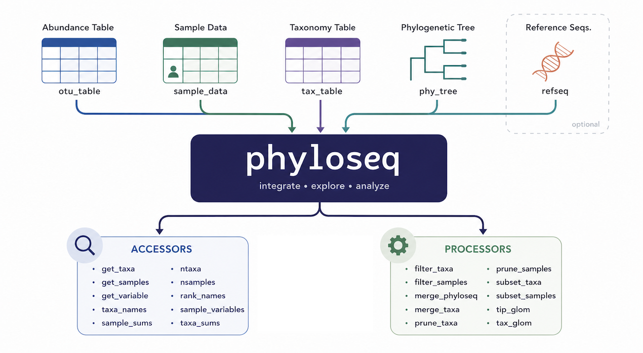
phyloseq is an R package that combines three data tables into a single, consistent object:

Component	Function	Description
OTU table	otu_table()	ASV × sample abundance matrix
Taxonomy table	tax_table()	ASV × taxonomic level annotations
Sample data	sample_data()	Sample-level metadata
Reference sequences	refseq()	The actual DNA sequences (optional)

Keeping everything in one object prevents accidental misalignment between tables and gives access to a rich set of analysis and visualisation functions.

7.2 Prepare metadata

We derive metadata directly from the sample names, which encode the experimental design (Group_Timepoint_Replicate).

# Parse sample names into experimental variables
metadata <- data.frame(
  SampleID = sample.names,
  row.names = sample.names,
  stringsAsFactors = FALSE
) %>%
  mutate(
    Group = case_when(
      startsWith(SampleID, "Lactobacillus") ~ "Lactobacillus",
      startsWith(SampleID, "Spontaneous")   ~ "Spontaneous",
      startsWith(SampleID, "Commercial")    ~ "Commercial",
      startsWith(SampleID, "Control")       ~ "Control",
      TRUE ~ "Unknown"
    ),
    Timepoint = case_when(
      grepl("_H24_", SampleID) ~ "H24",
      grepl("_H48_", SampleID) ~ "H48",
      grepl("_W1_",  SampleID) ~ "W1",
      grepl("_W2_",  SampleID) ~ "W2",
      TRUE ~ NA_character_
    ),
    Replicate = as.integer(sub(".*_R(\\d+)$", "\\1", SampleID)),
    IsControl = Group == "Control"
  )

# Verify that metadata rows match the seqtab rows
stopifnot(all(rownames(seqtab.nochim) %in% rownames(metadata)))

metadata

7.3 Build the phyloseq object

# Ensure tables are in the same order
metadata_matched  <- metadata[rownames(seqtab.nochim), ]
seqtab_matched    <- seqtab.nochim[rownames(metadata_matched), ]

stopifnot(all(rownames(metadata_matched) == rownames(seqtab_matched)))

otu <- otu_table(t(seqtab_matched), taxa_are_rows = TRUE)
tax <- tax_table(taxa)
sd  <- sample_data(metadata_matched)

ps <- phyloseq(otu, sd, tax)

# Store the actual DNA sequences in the phyloseq object
dna        <- Biostrings::DNAStringSet(taxa_names(ps))
names(dna) <- taxa_names(ps)
ps         <- merge_phyloseq(ps, dna)

# Rename ASVs to simple identifiers (ASV1, ASV2, ...)
taxa_names(ps) <- paste0("ASV", seq(ntaxa(ps)))

ps

phyloseq-class experiment-level object
otu_table()   OTU Table:         [ 1091 taxa and 29 samples ]
sample_data() Sample Data:       [ 29 samples by 5 sample variables ]
tax_table()   Taxonomy Table:    [ 1091 taxa by 6 taxonomic ranks ]
refseq()      DNAStringSet:      [ 1091 reference sequences ]

7.4 Filter unwanted taxa

16S amplification can co-amplify mitochondrial and chloroplast 16S-like sequences from plant and eukaryotic cells. These are not bacteria and must be removed before downstream analyses.

ps_filtered <- ps %>%
  subset_taxa(
    (is.na(Family)  | !grepl("mitochondria", Family,  ignore.case = TRUE)) &
    (is.na(Order)   | !grepl("mitochondria", Order,   ignore.case = TRUE)) &
    (is.na(Genus)   | !grepl("mitochondria", Genus,   ignore.case = TRUE)) &
    (is.na(Family)  | !grepl("chloroplast",  Family,  ignore.case = TRUE)) &
    (is.na(Order)   | !grepl("chloroplast",  Order,   ignore.case = TRUE)) &
    (is.na(Order)   | Order   != "Chloroplastida")
  )

cat("ASVs removed (mitochondria / chloroplasts):",
    ntaxa(ps) - ntaxa(ps_filtered), "\n")

ASVs removed (mitochondria / chloroplasts): 26 

7.4.1 Remove ASVs unclassified at Family level

For most downstream community analyses we require at least Family-level classification. ASVs that could not be classified even at this level are removed.

ps_final <- ps_filtered %>%
  subset_taxa(!is.na(Family) & Family != "")

cat("ASVs removed (unclassified at Family):",
    ntaxa(ps_filtered) - ntaxa(ps_final), "\n")

ASVs removed (unclassified at Family): 27 

cat("Final ASV count:", ntaxa(ps_final), "\n")

Final ASV count: 1038 

cat("Total reads in final dataset:", sum(sample_sums(ps_final)), "\n")

Total reads in final dataset: 4674036 

7.5 Taxonomic composition overview

tax_df  <- as.data.frame(tax_table(ps_final))
levels  <- c("Kingdom", "Phylum", "Class", "Order", "Family", "Genus")
total   <- ntaxa(ps_final)

tax_classif <- data.frame(
  Level = factor(levels, levels = levels),
  Pct   = sapply(levels, function(lv) {
    round(100 * sum(!is.na(tax_df[[lv]]) & tax_df[[lv]] != "") / total, 1)
  })
)

ggplot(tax_classif, aes(x = Level, y = Pct, fill = Level)) +
  geom_col(width = 0.7) +
  geom_text(aes(label = paste0(Pct, "%")), vjust = -0.4, size = 3.5) +
  scale_fill_viridis_d() +
  labs(title = "ASVs classified at each level (after filtering)",
       x = "Taxonomic level", y = "% of ASVs") +
  theme_minimal() +
  theme(axis.text.x = element_text(angle = 45, hjust = 1),
        legend.position = "none") +
  ylim(0, 110)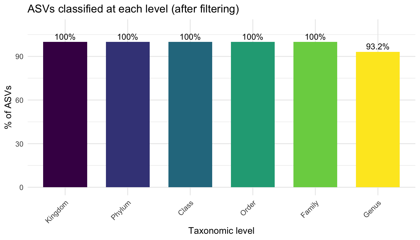

7.6 Filtering summary

cat("\n=== FILTERING SUMMARY ===\n")

=== FILTERING SUMMARY ===

cat("After denoising and chimera removal:      ", ntaxa(ps), "ASVs\n")

After denoising and chimera removal:       1091 ASVs

cat("After removing mitochondria/chloroplasts: ", ntaxa(ps_filtered), "ASVs\n")

After removing mitochondria/chloroplasts:  1065 ASVs

cat("After removing unclassified at Family:    ", ntaxa(ps_final), "ASVs\n")

After removing unclassified at Family:     1038 ASVs

cat("Samples in final dataset:                 ", nsamples(ps_final), "\n")

Samples in final dataset:                  29 

cat("Total reads in final dataset:             ", sum(sample_sums(ps_final)), "\n")

Total reads in final dataset:              4674036 

7.7 Export outputs

# Phyloseq object (for downstream analysis in R)
saveRDS(ps_final, "phyloseq_object.rds")

# ASV ID → sequence mapping
asv_sequences <- data.frame(
  ASV_ID   = taxa_names(ps_final),
  Sequence = as.character(refseq(ps_final)),
  stringsAsFactors = FALSE
)
write.csv(asv_sequences, "asv_sequences_map.csv", row.names = FALSE)

# ASV taxonomy + abundance table
asv_counts   <- as.data.frame(otu_table(ps_final))
tax_table_df <- as.data.frame(tax_table(ps_final))
write.csv(cbind(tax_table_df, asv_counts),
          "asv_tax_table.csv", row.names = TRUE)

# Sample metadata + per-sample read counts per ASV
sample_abundances <- as.data.frame(t(otu_table(ps_final)))
sample_metadata   <- as.data.frame(sample_data(ps_final))
write.csv(cbind(sample_metadata, sample_abundances),
          "samples_with_abundances.csv", row.names = TRUE)

cat("Outputs saved:\n")

Outputs saved:

cat("  phyloseq_object.rds\n")

  phyloseq_object.rds

cat("  asv_sequences_map.csv\n")

  asv_sequences_map.csv

cat("  asv_tax_table.csv\n")

  asv_tax_table.csv

cat("  samples_with_abundances.csv\n")

  samples_with_abundances.csv

7.8 What’s next?

The phyloseq_object.rds file is the starting point for all downstream analyses:

• Alpha diversity — species richness, Shannon entropy, Faith’s PD
• Beta diversity — Bray-Curtis or UniFrac distances, ordination (PCoA, NMDS)
• Differential abundance — DESeq2, ANCOM-BC, MaAsLin2
• Taxonomic bar charts — relative abundance at Phylum or Family level
• Network analysis — co-occurrence networks using SpiecEasi or SPRING

These topics are covered in the downstream analysis tutorial.