The typical genomics experiment can be divided in two main sections:
- The data reduction from raw FASTQ files to some count tables (bioinformatics)
- The statistical analysis of those count tables (inferential statistics)
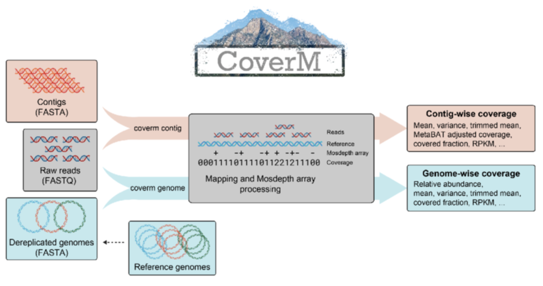
The mapping of reads against the co-assembly allows us to quantify the coverage of each contig in each sample.
We can use CoverM to produce an abundance table from a set of BAM files.
Installing CoverM
CoverM is easy installable from BioConda. We installed it in our “metadenovo” environment before, but you can create a dedicated environment for CoverM like this:
# Create and activate the environment
mamba create -n coverm -c conda-forge -c bioconda coverm
conda activate coverm

# Check installation
coverm --version
Running CoverM
We have a set of BAM files, each corresponding to the mapping of one sample against the co-assembly.
# Calculate coverage metrics for all contigs
coverm contig \
  -b ${bam_folder}/*.bam \
  -m count mean covered_fraction tpm \
  -o abundance_table.tsv \
  --exclude-supplementary \
  -t 8
Some explanations about the parameters used:
-
contig: is a subcommand which tells CoverM to calculate metrics at the contig level -
-b: specifies the input BAM files (you can specify multiple files, also using wildcards) -
-m: specifies the metrics to calculate, in this case:-
count: the number of reads mapped to the contig -
mean: mean coverage depth across the contig -
covered_fraction: proportion of contig covered by reads (0-1) -
tpm: Transcripts Per Million (normalized abundance)
-
-
-o: specifies the output file name -
--exclude-supplementary: excludes supplementary alignments from the calculations -
-t: number of threads to use
Output File
The output is a TSV file with the following structure:
| Column | Description |
|---|---|
| Contig | Contig identifier |
| {Sample} Count | Number of reads mapped to the contig |
| {Sample} Mean | Mean coverage depth across the contig |
| {Sample} Covered Fraction | Proportion of contig covered by reads (0-1) |
| {Sample} TPM | Transcripts Per Million (normalized abundance) |
Each sample gets one column per requested metric. In this case, with 3 samples and 4 metrics, you’ll have 13 columns total (1 for contig names + 3 samples × 4 metrics).
Note: Raw counts are the most useful value to perform statistical analyses, while TPM values are useful for a first “eyeballing” comparison of abundances between samples, as they account for both sequencing depth and contig length.